
This guide is for Excel users who are migrating to Google Sheets.
It lays out the differences between the two spreadsheet tools in detail.
You’ll learn what features are the same across both tools, what exciting new features exist in Google Sheets, and what you won’t find in Google Sheets.
This guide will help you determine what you might need to change with your current processes and workflows.
The goal of this guide is to get you up to speed with Google Sheets as quickly as possible, with the least amount of effort.
Highlighting
Google Sheets power features are denoted by a ?
Google Sheets limitations are marked with a ?
Contents
- Introduction
- Cloud Features
- Functions & Formulas
- Shortcuts
- Workings With Data
- Pivot Tables
- Charts & Dashboards
- Other Differences
- Macros, VBA & Apps Script
- Summary
Introduction
Change brings about strong emotions for everyone. Whether that’s feelings of fear or excitement, it can feel uncomfortable.
You probably have a strong bond with Excel built up through years of use. Years of building business solutions in Excel that you’re proud of.
In this guide, you won’t find opinionated debate as to which is a better tool, or why one is great and the other one not. That won’t help you with the migration process.
Rather, the goal with this guide is to make you feel excited about using Google Sheets.
High-Level Comparison
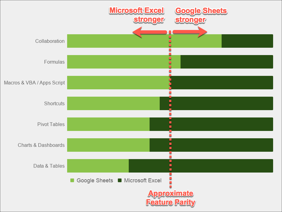
In Summary
- Both are phenomenal tools, when used in the right hands
- For probably 80-90% of regular spreadsheet scenarios, either will suffice
- Excel still has significant strengths in certain areas, especially data analysis, big datasets and complex charting
- Google Sheets continues to close the gap
For general spreadsheet work, like working with regular datasets, formatting tables, making lists, tracking inventory, there’s little to pick between the two programs.
It may take a little while to get used to operations, shortcuts and menus in Sheets, but at the end of the day, it’s still a spreadsheet program and similar in a lot of ways.
Who Is This Guide For?
This guide is aimed at Excel users, like business analysts or finance teams at medium to large enterprises, who are migrating from Microsoft Office to G Suite.
Keep An Open Mindset
Embrace this opportunity to learn.
There may be some constraints to what you can do. But constraints breed creativity.
It’s a chance to improve workflows and streamline processes. To re-imagine your work.
There will be new features to explore. Features that will delight you.
You need to open your mind to new possibilities.
Objections To Google Sheets
If you’re reading this paragraph, you may not be happy about the fact that you’re migrating to Google Sheets from Excel.
You’ve probably had these thoughts in your mind or heard them from colleagues:
- I’m an expert with Excel and don’t want to learn something new
- Google Sheets is a “toy spreadsheet” and not capable enough
- We have decades worth of experience and know-how encapsulated within our Excel spreadsheets
- We’ve built custom software with Excel and VBA that is crucial to our team
- I know VBA but don’t have a clue whether Google Sheets has macros or scripting available
- Google Sheets can’t handle the size of the datasets we have in our Excel files
- Etc.
These are valid concerns. I’m not here to tell you otherwise.
But if you’re migrating to Google Sheets, and want solutions, read on with an open mind.
CLOUD FEATURES
Cloud Features
Browser Based
Google Sheets is a web application that runs in your browser, think of it like a very sophisticated website. It’s created with the Javascript programming language and the files are stored on Google’s servers.
Contrast this to Excel, which works locally on your desktop (note: Excel 365 is their online version). Excel is written in C++ programming language and executes on your local machine, which is one reason why it’s faster.
Each Google Sheet is a single file in the cloud, with full version control. This means you no longer need to keep multiple copies of the same spreadsheet, with each person saving a new copy and adding their thoughts.
You don’t have to worry about compatibility across devices. Everybody uses the same version of Google Sheets so your file will open for everyone else.
All that collaboration happens simultaneously in the cloud. Collaborating with colleagues in a Google Sheet in real-time and chatting in the sidebar will transform your workflows.
Sharing & Collaboration
Collaboration is Google Sheets’ superpower. It’s been built from the ground up with collaboration in mind.
Sharing is super easy, and you have full control over what other people can do with the Sheet.
You can easily share a Google Sheet by clicking the button in the top right, where you’ll find options to share with others via email or shareable link. You also have control over the kind of access: view only, comments allowed or full editing access.
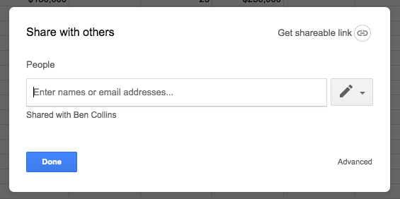
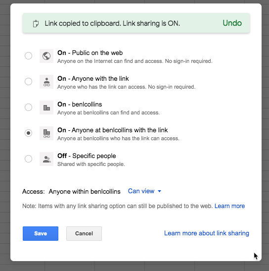
From the Share box, you can also grab a shareable link (top right of the share box). You can restrict the file to staying within your G Suite organization or sharing externally. You also have control over the kind of access: view only, comments allowed or full editing access.
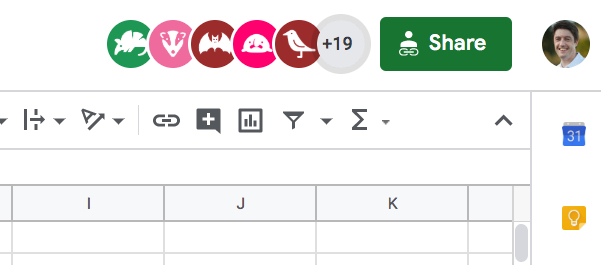
If you share a Sheet with others via email, you’ll notice their name and avatar show up in the Sheet whenever they’re active.
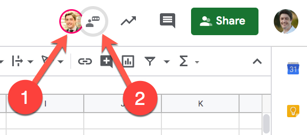
Clicking on someone’s avatar (1) will move your cursor to wherever that person is active in the Sheet. You can also click the chat box (2) and being chatting with others, directly in the Sheet.
If you’ve shared the Sheet publicly via a shareable link and others start viewing, you’ll see those people show up as anonymous animals. No, really ?♂️
Microsoft have introduced Office 365, their cloud based suite of productivity tools. Excel 365 has collaboration built-in too, but many agree it’s not quite as seamless as Google’s implementation yet.
For more information about sharing files with Google Sheets, see:
Notification Rules
Do you collaborate with colleagues in Google Sheets?
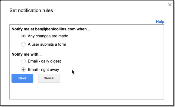
Stay informed of changes to a Google Sheet by setting Notification Rules to send you an email.
You’ll find it under this menu: Tools > Notification rules…
Here you can decide what should trigger a notification and how they should be delivered (immediately or a daily summary):
Never miss an update to your Google Sheets again!
Google Sheets And Excel Compatability
Importing From Excel
You can import Excel files directly into your Google Sheets and convert them into Google Sheets.
Or, you can work on Excel files from the Google Sheets interface without doing the conversion.
This brings the collaboration benefits of Google Sheets to Excel files and streamlines workflows by eliminating the need to convert file types. If you work with partners or other team members who still use Excel, then this feature will make collaboration seamless.
To open an Excel file in Google Sheets without converting it, double-click the Excel file in your Google Drive. From the preview window, click the Open in Google Sheets button at the top.
In Google Sheets, it’ll look like a regular Google Sheet, but you’ll see a .xlsx (or .xls, xlsm, .xlt) label to indicate it’s still an Excel file.
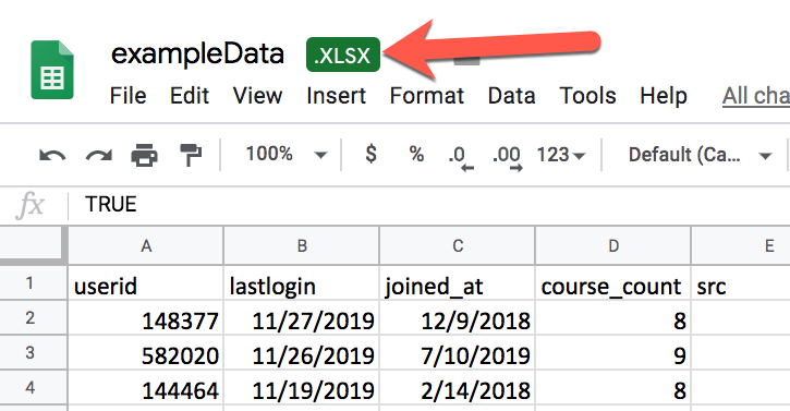
In this configuration you can work on the file and any changes will be saved into the original Excel file.
However, not all the elements of an Excel file can be transferred into a Google Sheet:
- Excel slicers will not be imported
- Macros or other VBA scripts in Excel will not be imported.
You’ll have to recreate slicers and any scripts anew in Google Sheets.
Offline Access
You can work offline with Google Sheets but there are some important points to note:
- You can view, edit and create Google Sheets offline…
- …however, you need to manually change settings to allow offline access before you go offline
- You also need to be using the Chrome browser and have the Google Docs Offline extension installed
- Changes to offline Google Sheets are saved locally and synced back to the cloud when you go back online. This all happens automatically.
- Macros, custom functions and Apps Script are not available (since they all run on Google servers and require an internet connection to run)
For more information about working offline, see:
? Publish To Web
Publish your Google Sheets to the web, so you can easily share online or embed into other websites.
This option is found under the File > Publish to the web
For more information about publishing to the web, see:
FUNCTIONS & FORMULAS
Functions & Formulas
Excel power users often worry that the functions available in Google Sheets are not as advanced or numerous.
Well, you’ll be pleasantly surprised to not only find that the vast majority of Excel functions are available directly in Google Sheets, but that Google Sheets also has its own native functions that are incredibly powerful and useful.
This means you can construct formulas in Google Sheets that are as complex as anything in Excel. Not every single function or formula will transfer across directly, but usually you’ll find a way to do it.
Google Sheets has nearly 500 functions. You can find a list of the Google Sheets functions here.
Excel has slightly fewer, around 478. You can find a list of the Excel functions here.
Note that both spreadsheets are constantly updating their function lists, so anytime one spreadsheet gets a new function, you can expect it to appear in the other at some point in the future.
If you want to explore these functions within your Google Sheet, you can use this IMPORTHTML formula to import them into a Google Sheet:
=IMPORTHTML( A1 , "table" , 1 )
where the value of A1 is the URL from the function links above.
Google Sheets vs. Excel Function List Template
(Note: if you’re unable to open this link and are prompted to request permission, it’s because your organization has not whitelisted my G Suite domain, benlcollins.com. You may be able to ask your G Suite administrator about it. In the meantime, you can also open the link in an incognito tab (right click the link and choose Incognito Tab) to view the contents.)
Below, I’ll introduce some of the killer functions that are unique to Google Sheets.
? The QUERY Function
The QUERY function is arguably the most powerful and versatile spreadsheet function ever created. It does the work of multiple other functions and can replicate a lot of the functionality of Pivot Tables in formula form.
It uses a special syntax, very similar to the SQL language that databases use to manipulate data.
It’s incredibly powerful because you can filter, sort, modify and run calculations on entire datasets with a single formula.
The syntax looks like this:
=QUERY( countries , "SELECT C, count(B) GROUP BY C" , 1 )Where “countries” is a named range in the dataset and the B, C letters refer to the columns being selected.
Further reading on the QUERY function:
- Google Sheets Query function: The Most Powerful Function in Google Sheets
- How to add a total row to a Query Function table in Google Sheets
- Filtering with dates in the QUERY function
- Lessons 14 and 15 of the free Advanced Formulas in Google Sheets course
? Array Formulas
Whereas a normal formula outputs a single value, array formulas output a range of cells!
The syntax for Array Formulas is slightly different between Excel and Google Sheets.
Both can be entered with the Ctrl + Shift + Enter action, but where the Excel formula then shows with a pair of curly braces around it, the Google Sheets formula has the ArrayFormula function inserted.
Compare the Excel version:
{ =SUM( A1:A5 * B1:B5 ) }
With the Google Sheets version:
=ArrayFormula( SUM( A1:A5 * B1:B5 ) )
Both Excel and Google Sheets support Arrays (structures that hold a collection of values). Arrays are constructed with curly brackets.
Commas separate the data into columns on the same row.
Semicolons creates a new row in your array.
This formula, entered into cell A1, will create a 2 by 2 array that puts data in the range A1 to B2:
= { 1 , 2 ; 3 , 4 }
For more information about the ArrayFormula, see:
- How do array formulas work in Google Sheets?
- Lesson 17 of the free Advanced Formulas in Google Sheets course
? The IMPORTRANGE Function
The IMPORTRANGE function is unique to Google Sheets. There’s no equivalent in Excel, because you can link to other desktop files through a regular file link.
However, since Google Sheets is entirely in the cloud, it needs to have a robust way to access data in other Google Sheets.
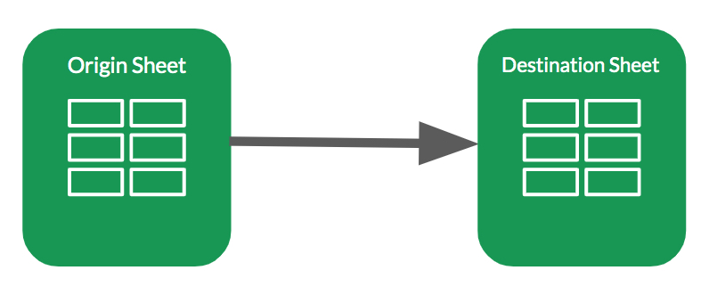
The IMPORTRANGE function is the only way to connect Google Sheets and bring data from one into another:
The formula syntax is:
= IMPORTRANGE( spreadsheet_url , range_reference )
When you first connect two Sheets, you have to authorize the IMPORTRANGE function. This has to be done before you wrap it inside other functions, lest you get an error message.
For more information about the IMPORTRANGE function, see:
- Lesson 18 of the free Advanced Formulas in Google Sheets course
- The IMPORTRANGE documentation from Google
The Other IMPORT Functions
In addition to the IMPORTRANGE function, for importing data from one Google Sheet into another, Google Sheets has four other IMPORT functions:
- IMPORTDATA, which imports data from a given URL in .csv or .tsv format into Google Sheets
- IMPORTFEED, which imports a RSS or ATOM feed into Google Sheets
- IMPORTHTML, which you saw in the function introduction section, for importing data from HTML lists or tables on a webpage into Google Sheets
- IMPORTXML, which imports data from structured data types at a given url
They can be used to import data from websites, CSV or TSV files or even RSS feeds into your Google Sheet. They’re extremely powerful.
For example, with the IMPORTXML function you can import information directly from webpages into Google Sheets.
Here, I extract the number of followers from Google’s Twitter profile:
=QUERY( IMPORTXML( "https://twitter.com/Google" , "//span[@class='ProfileNav-value']/@data-count" ) , "limit 1 offset 2" )The inner IMPORTXML function returns a packet of data, which the wrapper QUERY function parses to extract just the number of followers.
For more information about how to use these IMPORT formulas to retrieve web data, see:
- Using Google Sheets as a basic web scraper
- How to import social media statistics into Google Sheets: The Import Cookbook
? The REGEX Functions
The REGEX functions – REGEXMATCH, REGEXEXTRACT, REGEXREPLACE – bring the phenomenal power of regular expression to your Google Sheets.
It means you can go way beyond the text formulas like SEARCH, FIND, LEFT, MID, etc. to parse strings and match data.
For example, this formula will extract a value from a string in A1:
=VALUE( REGEXEXTRACT( A1 , "[0-9,]+" ) )And this one will extract an email address from a string in A1 (image shows A7):
=REGEXEXTRACT( A1 , "[a-zA-Z0-9_\.\+-]+@[a-zA-Z0-9_\.\+-]+" )
Be warned though, regular expression is a challenging syntax to learn.
For more information about REGEX functions in Google Sheets, see:
- Lesson 20 of the free Advanced Formulas in Google Sheets course
- Google’s re2 regular expression syntax (used in the REGEX functions)
The Google Finance Function
The Google Finance function allows you to bring financial information, like stock ticker prices, into your Google Sheets easily. It fetches current or historical securities information from Google Finance.
For example, this function imports daily stock prices for Google:
=GOOGLEFINANCE( "GOOG" , "price" , TODAY() - 30 , TODAY() , ”DAILY” )For more information about the GOOGLEFINANCE function, see:
The Google Language Functions
Take advantage of Google’s language translation capabilities and easily translate languages inside your Google Sheets with the GOOGLETRANSLATE and DETECTLANGUAGE functions.
For example, the Google Translate function can be used to translate text in cell A1 into English with the following syntax:
=GOOGLETRANSLATE( A1 , "auto" , "en" )The “auto” reference defers to Google to automatically detect the language.
For more information about the Google Language functions, see:
? The Sparkline Function
Sparklines in Google Sheets have been implemented in a different way to Excel. And I think it’s superior in some ways.
Sparklines in Google Sheets are created with the SPARKLINE function, which makes it easy to build formulas that output the miniature sparkline charts in your cells.
Here’s an example Sparkline function:
=SPARKLINE(A1:A20 , { "charttype" , "column" ; "highcolor" , "red" })The syntax is a little complex and takes some time getting used to, but it’s no more challenging than other advanced formulas like the QUERY function.
This formula above outputs a miniature column chart inside a single cell, with the highest value highlighed as the red bar:

For more information about the SPARKLINE function, see:
- Everything you ever wanted to know about Sparklines in Google Sheets
- Lesson 21 of the free Advanced Formulas in Google Sheets course
- A complex sparkline example: Google Sheets Formula Clock
The IMAGE Function
The IMAGE function, unique to Google Sheets, inserts an image into a cell. The image is then locked into that cell and acts like any other element in a cell would, i.e. it will move with the cell if you insert rows or columns, it’ll become hidden if you hide that row etc.
The image needs to be accessible at a URL, excluding those behind password walls or ones hosted on Google Drive. Optionally, you can specify how to size the image once it’s embedded into your cell.
The IMAGE function is a nice way to add context to your Sheets. For example, you can include your company logo inside Sheets. You could add client logos to a contacts database. You could add useful diagrams to reference Sheets to help add context to calculations. Etc…
The syntax for the IMAGE function is:
= IMAGE( "https://www.google.com/favicon.ico" )which looks like this in your Google Sheet:
The optional sizing arguments are added after the image URL.
Use the MODE to set the aspect ratio and image behavior, and the optional HEIGHT and WIDTH to set the size.
= IMAGE( "https://www.google.com/favicon.ico" , 4 , 100 , 100 )The 4 indicates a custom size of 100px by 100px.
Note, you can also insert images directly into cells from the Insert menu. There’s no requirement to use a URL, which means you can add images from your local drive.
You find this image feature under the menu: Insert > Images > Image in cell
For more information about the IMAGE function, see:
- The IMAGE function documentation from Google
- Formula Challenge #1: Repeating Images with Array Formulas
The Hyperlink Function
The Hyperlink function turns a cell into a clickable link to an external URL, which opens in a new tab of your browser.
It’s a really useful function, for everything from adding links to other Google Docs (e.g. process notes), linking to external resource websites, client websites, etc.
The Hyperlink function is easy to understand. It takes two arguments: 1) the URL, and 2) the text to display in the cell:
=HYPERLINK( "https://www.benlcollins.com/" , "Ben Collins Website" )which looks like this in your Google Sheet:
Now, suppose you want to extract URLs from hyperlinks in your Google Sheet, how does one do that?
Firstly, turn the hyperlink into text so that the URL is showing, with this formula (assuming the hyperlink formula is in cell A1):
= FORMULATEXT( A1 )
Next, wrap this with a REGEXEXTRACT function, which extracts just the URL:
= REGEXEXTRACT( FORMULATEXT( A1 ) , """(.+?)""" )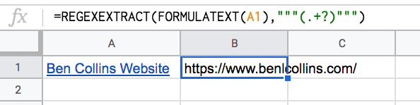
Now you can drag this formula down the column if you have more hyperlinks to extract, which is much quicker than doing it manually!
Internal Hyperlinks
Note: You can also add hyperlinks to different tabs or even directly to individual cells within your Google Sheets.
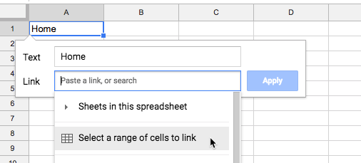
They’re super easy to create. You don’t even have to write any formulas yourself. Simply:
- Right click on the cell that you want to turn into a clickable hyperlink
- Click “Insert link”
- Choose either “Sheets in this spreadsheet” or “Select a range of cells to link”
That’s it!
Here’s a few examples of how you could use this:
- Add a Home button to every tab in your Sheet so you can quickly get back to the first tab
- Create a “table of contents” for your Sheet
- Link to important calculation cells so they can be easily accessed
Other Functions Unique To Google Sheets
This is not an exhaustive list, but here are a few other notable Google Sheets only functions:
- The SPLIT function
- ISDATE
- ISEMAIL
- ISURL
? What Functions Are Missing From Google Sheets?
Excel has some functions that Google Sheets does not:
- The new XLOOKUP function (at the moment anyway!)
- Cube functions
- INFO(), SHEET() and SHEETS()
- Some esoteric statistical functions
(This is not an exhaustive list!)
? Formula Auditing
Unfortunately, the formula auditing capabilities of Google Sheets are severely limited compared to Excel. There are only a few techniques available, which I detail here.
Function Helper Pane
The function helper pane gives information about the function you are editing. If you’re dealing with a formula with multiple functions, then it refers to the function that is active per the location of your cursor.
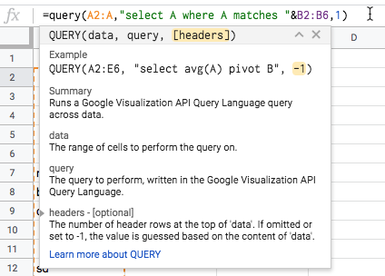
You can press the “X” to remove the whole pane if it’s getting it the way. Or you can minimize/maximize with the arrow in the top right corner.
The best feature of the formula pane is the yellow highlighting it adds to show you which section of your function you are in. E.g. in the image above I’m looking at the “[headers]” argument.
There is information about what data the function is expecting and even a link to the full Google documentation for that function.
If you’ve hidden the function pane, or you can’t see it, look for the blue question mark next to the equals sign of your formula. Click that and it will restore the function helper pane.
Trace Precedents Equivalent
Pressing the F2 key enters the formula view of a cell that contains a formula.
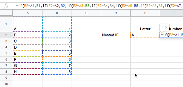
Google Sheets highlights ranges in your formula expression and in your actual Sheet with matching colors. It applies different colors to each unique range in your formula.
This is the equivalent of trace precedents in Google Sheets.
However, F2 also accesses another helpful feature. If you position your cursor over a data range reference inside your formula and press the F2 key, it will highlight that range of data for you, even if it’s in a different tab of your Google Sheet:
You can also view formulae by clicking on the View > Show formulas or use the shortcut Ctrl + `
There is also the function FORMULATEXT, which returns the formulas as a text string.
GoTo Equivalent
Excel has a useful feature called GoTo, which lets you easily jump around your spreadsheets and find specific information or items.
Google Sheets does not have this functionality, but we can use alternative techniques to achieve the same goal.
Suppose your Google Sheet is full of formulas and you want to see where they all are, so you can check them. You don’t want to simply look through the Sheet because you might miss some.
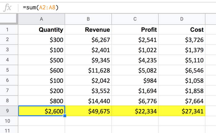
Instead, use conditional formatting to highlight them all.
Click on the box in the top left corner, between the column A and the row 1 headings. This will highlight your entire Sheet.
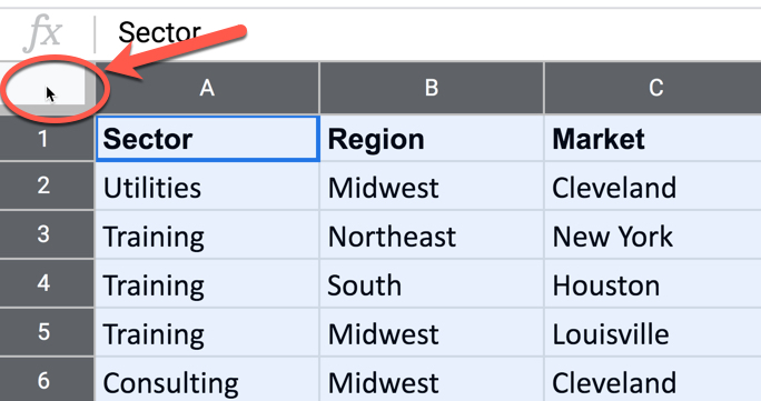
Then choose Format > Conditional Formatting from the menu
Select “Custom formula is” under the Format rules.
Set the formula to:
=ISFORMULA( A1 )
Change the formatting style if you wish. I like to use a bright yellow.
Click Done and all the formulas in your Sheet will be highlighted, making them much easier to see.
You can use this same technique with other conditional formatting rules like ISERROR to find all your errors.
For more information about formula techniques, see:
SHORTCUTS
Shortcuts
Microsoft Excel does have a more comprehensive suite of shortcuts available, but what most people probably don’t realize is that Google Sheets has a surprising number of its own shortcuts.
Of course, even despite this, the big challenge here is to rewire years of muscle memory for new shortcut key combinations. Unfortunately that is just going to take time and feel awkward for a while.
To see all of the available shortcuts in Google Sheets, go to the help menu, Help > Keyboard shortcuts, or press Ctrl + / (PC/Chromebook) or Cmd + / (Mac).
Here are 5 of the most popular shortcuts in Google Sheets:
1. Clear All Formatting in a cell or range
Mac: ⌘ + \
PC: Ctrl + \
2. Insert the current date in a cell
Mac: ⌘ + ;
PC: Ctrl + ;
3. Select all the data in a table
Mac: ⌘ + A
PC: Ctrl + A
4. Find and Replace
Mac: ⌘ + Shift + H
PC: Ctrl + H
5. Open the drop-down menu on filtered cell
Mac: Ctrl + ⌘ + R
PC: Ctrl + Alt + R
Today, I challenge you to use keyboard shortcuts.
It might feel clumsy at first, but persevere and it’ll pay off in spades as you become more efficient in your work.
For a complete, online list of shortcuts for Google Sheets, see:
? Instantly Create A New Google Sheet
Type sheet.new or sheets.new into your web browser to instantly create a new Google Sheet (if you’re not logged into your Google account you’ll be prompted to do that first).
This also works for Google Docs, Forms, Slides and some other G Suite apps.
The new Google Sheet is created in the root directory of your Google Drive.
If you want to create a new Google Sheet in a specific folder of your Google Drive, then there is a shortcut for that.
Press Shift + S when you’re inside the folder to create a new Google Sheet there.
WORKING WITH DATA
Working With Data
Sorting
Excel has more sophisticated Sorting options than Google Sheets.
In Google Sheets, you CANNOT:
- Sort Left to Right
- Make Sort case sensitive
Data in a Google Sheet can be sorted from the Data menu (or by using a function like SORT or QUERY):
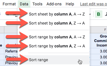
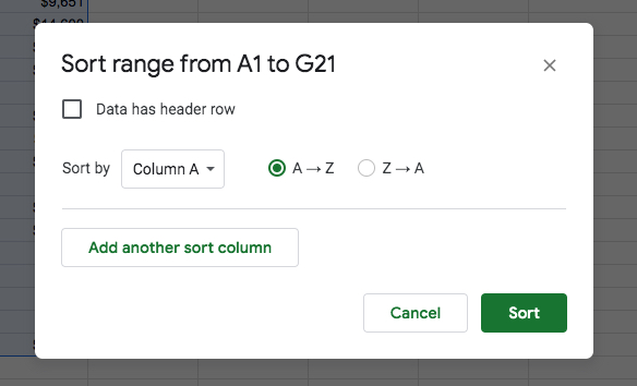
Clicking Sort Range brings up the sort options available in Google Sheets:
Filters
Excel has more sophisticated Filter options than Google Sheets.
However, Google Sheets has a powerful feature called Filter Views (see below) , which Excel does not have.
In Google Sheets, you CANNOT:
- Click on a cell and filter by that cell’s value. You can only access filters from the column headings in Google Sheets.
- Clear all filter settings in one go (you either have to remove them one by one, or remove the Filter altogether an re-add it)
You add filters to Google Sheets via the Data menu or the filter icon in the toolbar ![]()
This gives you all the standard options for sorting and filtering: by value (e.g. all “Customer A” in the column) or by condition (e.g. all values over 100).
? FILTER Views
Filter Views are unique to Google Sheets. It’s an elegant solution to the issue of multiple people are looking at the same table in a Google Sheet and someone applies a filter. Everyone’s view changes.
It allows different users of a Google Sheet to see their own filters on a dataset, without affecting other users view of the dataset.
The answer is to save your filter set as a Filter View, give it a name and then you can use it without disturbing others viewing the same dataset.
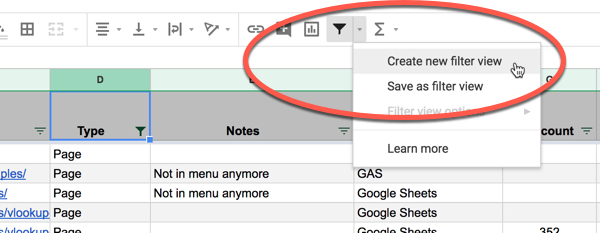
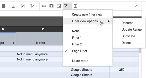
If you already have a filter setup, then you can just save that as a Filter View and give it a memorable name. Alternatively, you can create a new filter under this menu too:
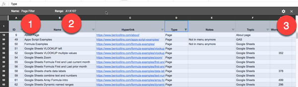
Your Filter View will then show up, with a dark grey box around it.
Here you can rename it (1), adjust the range (2) and update, delete or duplicate it (3). The X on the right side allows you to also close the Filter View:
Once you have a Filter View saved, it’s available to use again under the filter button menu, along with the Filter view options menu:
The major benefit of these Filter Views is that other people working with this dataset in the same Sheet are unaffected. They can continue to see the whole dataset or create their own Filter Views, independent of yours.
Another benefit of course, is that you can save more complex filters using multiple columns to easily return to them.
For more information about Filters and Filter Views in Google Sheets, see:
- The Sort & Filter your data documentation from Google
- Google Sheets Sort And Filter By Color With Apps Script
? Tables
Excel has the very powerful Excel Tables feature, which brings a host of benefits, including column name referencing, auto-fill down and auto-formulas. It’s a huge boon when working with datasets.
Google Sheets does not have this feature.
Google Sheets only has an Alternating Colors option for tables, which will apply color banding automatically to new rows or columns. This is purely a formatting feature though, and does not facilitate any of the referencing or other auto-complete features of Excel Tables.
Named Ranges
Google Sheets has the Named Ranges feature, so you can name your ranges as you would in Excel. You can then use these Named Ranges in formulas, but not in Pivot Tables or as Chart data.
=SUM( someNamedRange )
Excel’s Named Range feature is more sophisticated.
Excel permits formulas in named ranges, which is a very powerful technique to create dynamic arrays that can be used to create dynamic charts for example.
You can also use named ranges in Pivot Tables and Charts in Excel.
Although formulas are not accepted in named ranges in Google Sheets, you can still create dynamic named ranges using a cunning trick with the INDIRECT function. Essentially you can create a string version of your formula, make that formula cell a named range and then refer to it with the Indirect function.
Read more: How to create dynamic named ranges in Google Sheets
Geographic And Stock Datatypes
Earlier this year Microsoft added two new, rich datatypes to Excel: geographic data and stock data.
When you use either of these datatypes you can easily augment that data with related information. For example, if you have a list of US States then you can easily add their populations or areas (or a multitude of other measures) with a few clicks. Same for stock information.
Google does not have these rich datatypes.
However, you can use the GOOGLEFINANCE function to import a variety of information about stocks.
For geographic information, you’re stuck using formulas or copy-pasting data into your Sheets.
Data Analysis
Goal Seek
In October 2019, Google released their own Goal Seek add-on for Google Sheets.
Goal Seek is an Add-On, which means you need to add it to your Google Sheet before you can use it.
Search for “Goal Seek” in the Add-Ons marketplace, found under the menu Add-ons > Get add-ons
It can be used to run the same types of sensitivity calculations you’d run in Excel.
For more information about the Goal Seek add-on and example calculations, see:
Solver
Whilst there is no native Solver feature or official add-on from Google, there are a number of third-party solver add-ons available. However, they are not as powerful or fully featured as Excel, and are slow to work with bigger datasets.
For more information about third-party solver add-ons, see:
What-if Analysis
Google Sheets does not have an equivalent to the what-if analysis feature.
? Get & Transform (Power Query)
Google Sheets does not have a native equivalent to Get & Transform.
If you’re using Google Cloud products alongside Google Sheets, as part of your data analysis pipeline, then you’ll find that Data Prep offers similar functionality.
In Google Sheets itself, there are various ways of importing data (e.g. File > Import, IMPORT functions, Apps Script). Then you can use functions to do any data wrangling.
? Power Pivot
Google Sheets does not have an equivalent to Power Pivot.
? Excel Data Model
Excel 2013 introduced a new in-memory analytics engine called the Data Model, and every workbook has one.
Using this Data Model, you can tell Excel how different data tables are connected and build an analytics cube from them. No more messing about building intermediate tables with VLOOKUPs and the like.
Google Sheets does not have an equivalent to the Excel Data Model.
For joining tables in Google Sheets, you can either use formulas, write an Apps Script program or use third-party add-ons.
There are two useful add-ons for working with multiple tables:
Sheetgo is an add-on for managing workflows across multiple Google Sheets and for stacking tables atop one another (like a vastly more featured and robust IMPORTRANGE tool).
Merge Sheets from Able Bits is an add-on for merging tables from different tabs within a single Google Sheet. It’s easier to setup and use than having hundreds of VLOOKUPs.
? Big Data
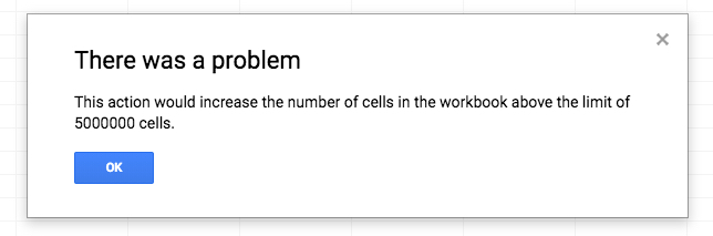
Google Sheets has an upper limit of 5 million cells.
If you do something that will take you past this limit (e.g. adding new rows or a new Sheet), you’ll see this error message:
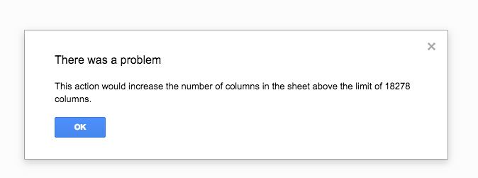
Google Sheets has a maximum number of columns allowed of 18,278.
If you do something that would take you past this limit, you’ll see the following error message:
Within a single cell, there’s a maximum string length of 50,000 characters (enough for approximately 500 average sentences, or about 162 Tolstoy sentences).
In Sheets, once you get beyond roughly 100,000 rows of data, you’ll find the performance noticeably slows.
For more information about slow Google Sheets, see:
Connecting To External Databases
Google Sheets has a native data connector to join to a BigQuery database.
? Connected Sheets will take this connector a step further by letting you use regular Google Sheet features like functions and pivot tables with data in BigQuery. This is currently in beta testing phase.
In addition, Google has a number of connectors or add-ons available for the popular enterprise software platforms, including: SAP, Salesforce and Zendesk.
Connections to other databases are possible using third-party tools (like Supermetrics) or creating your own custom connectors using Apps Script with the JDBC connector.
For more information on connecting to databases, see:
- Connected Sheets information from G Suite blog
- Information about the SAP ERP and Google Sheets integration
- Information about the Salesforce Data Connector Add-On
- Information about the Zendesk Data Connector Add-On
- Apps Script JDBC connector for external databases
- Google Sheets Data Connector from Supermetrics
? Working With OLAP Data
Online Analytical Processing (OLAP) is a category of data warehousing optimized for analyzing large amounts of data as quickly and efficiently as possible.
OLAP databases differ from traditional, transactional databases because they’re designed for reporting and data analysis. Data may be appended to OLAP databases but is rarely edited or deleted.
Although there are some connectors for OLAP Cubes and Google Sheets (e.g. here), it’s not common.
Google BigQuery shares some similarities with OLAP databases. BigQuery is designed for super fast processing of huge datasets.
And BigQuery integrates natively with Google Sheets, using the data connector and Connected Sheets mentioned above (under the previous subhead Connecting to External Databases).
PIVOT TABLES
Pivot Tables
This is certainly one area around which there’s still a lot of misconception.
Pivot tables in Google Sheets and Excel are built on the same fundamental premise: that you can take big datasets and transform them into summary reports with just a few clicks. Without a doubt, they’re the single most powerful feature of spreadsheet programs.
Of course, the implementation varies dramatically, so they look and feel a little different. But if you can use an Excel pivot table comfortably then you’ll have little problem working with pivot tables in Google Sheets.
Google Sheets pivot tables are powerful and have a lot of the standard functionality of their Excel counterparts.
They were updated in a major way in 2018 with features like grouping, which made them dramatically more powerful.
In 2019, slicers were introduced to allow quick filtering of pivot tables and introduce a new era of interactivity for Google Sheets reports.
However, they are still not as powerful for data analysis as their Excel counterparts.
Pivot Table Features In Google Sheets
Pivot tables in Google Sheets are advanced and capable of sophisticated analysis.
The following features are all available in Google Sheets pivot tables:
- Calculated Fields
- Grouping by Date fields
- Grouping values into intervals (Pivot Group Rule)
- Custom Grouping by highlighted values
- Sorting
- Filtering
- Pivot tables can be created in a new tab or an existing tab
- Double click to bring up records for a specific datapoint in a pivot table
- You can access and modify pivot tables with Apps Script (see the pivot table class)
In addition, there are some features unique to Google Sheets pivot tables that you’ll come to appreciate:
- You can have the same field as a Row heading and as the FILTER option
- You can use custom formulas in a pivot table filter, which is very powerful
- You can change column headings and calculated field names by simply typing over the existing headings in the pivot table in your Sheet
- The top left cell of a pivot table in Google Sheets is like an “anchor” cell. You can copy a pivot table quickly by just copying and pasting this single cell
Grouping Examples
There are three powerful ways to group your row data in pivot tables for dates, numeric data and text data.
Note: If you want to remove the total for a grouped set, you have to do this before doing any grouping. Unchecking the total on a grouped row/column also removes the grouping (which may cause problems as your table suddenly expands).
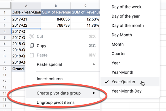
Grouping Dates
If you add a date into the Row option for your pivot table you can right click the dates and select Create pivot date group to get the date grouping you want (not all shown in this image).
Grouping Numeric Values With The Pivot Group Rule
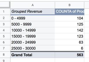
If you add a numeric data into the Row option for your pivot table you can right click on the number values, choose Create pivot group rule and then set the custom interval you want.
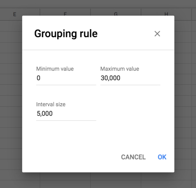
A pivot table with this Pivot Group Rule applied will look like this:
Grouping Text Values
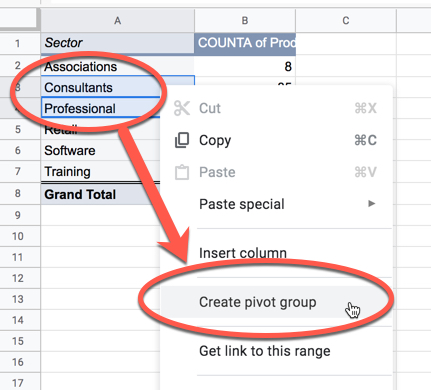
If you add text data into the Row option for your pivot table, you can highlight text values into a group (hold down Ctrl), then right click and select Create pivot group to group these items together.
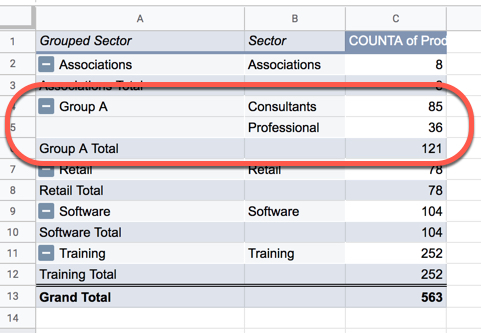
A pivot table with this Pivot Group Rule applied will look like this:
? What Google Sheets Pivot Tables Are Still Missing
Excel pivot tables have been around a lot longer, and they have a lot more features that have not made it into Google Sheets yet.
The key shortcomings of Google Sheets pivot tables are:
- You have to type the name of existing fields (the column headings from the dataset) in calculated fields. There is no option to click on their names from a list
- Filters do not appear in the Sheet above the pivot table like Report Filters do in Excel (in Sheets, they’re only accessible through the editor sidebar)
- No Row or Column label filters on Google Sheets pivot tables
- No Top 10 filter functionality in Google Sheets pivot tables
- Excel date filtering has many more pre-defined options available
- No calculated items in Google Sheets pivot tables
- No custom list sorting in Google Sheets pivot tables
- No option to list the calculated formula details for Google Sheets pivot tables
- No Pivot Charts in Google Sheets (see below)
- No Data Models in Google Sheets (see below)
Pivot Charts
Pivot Charts are not available in Google Sheets. ?
However, if you’re clicked anywhere in a pivot table and then you insert a chart (Insert > Chart menu), it will be “linked” to this pivot table and expand or contract as rows are added to or removed from the pivot table.
Note that adding new fields to the pivot table will not propagate through to the chart though, and the chart will require manual updating.
Data Models
There are no Data Models in Google Sheets. ?
Without the Data Model architecture, you can’t combine disparate datasets directly into single pivot table. You have to create an intermediate table the old fashioned way with functions like VLOOKUP.
See the previous Data Analysis section for more details.
Slicers
In Excel, slicers are graphical versions of report filter fields for pivot tables.
In Google Sheets, you can add slicers to data tables and/or pivot tables.
It’s critical to understand how slicers are implemented in Google Sheets, because it’s not intuitive.
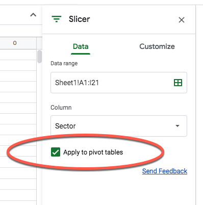
You can’t connect slicers to specific pivot tables the way you do in Excel. Instead it’s all based on the sheet (tab) that the slicers reside in.
If you add a slicer to a data table and then apply a filter, it will hide rows of data in that table. If you choose the “Apply to pivot tables” option, then the slicer will also apply to all the pivot tables in this tab only.
Slicers apply only within the sheet (tab) they’re in.
If you want to have slicers operating on different pivot tables (and charts) then they need to be in separate sheets (tabs).
Google Sheets slicers can have custom colors and fonts.
This is how the slicers operate in Google Sheets:
Slicers are definitely more basic in Google Sheets than in Excel, but they’re much easier to setup and understand.
Anyone with access to the Sheet can see and adjust a slicer. When you apply a filter with a slicer, any changes are only visible to you (unless you set them as default, in which case they’ll be applied for everyone that has access to the Sheet).
Everyone with access to the Sheet can see slicers, but only users with edit access can add or remove new slicers.
Key Differences
- Google Sheets does not have timeline slicers like Excel
- You cannot used grouped dates in slicers in Google Sheets, only data from the underlying table
- You cannot create multi-row or -column layouts with slicers in Google Sheets. They’re restricted to the filter style view.
- You cannot restrict slicers to specific pivot tables only
- Slicers are not imported into Google Sheets when you import an Excel file
For more information on pivot tables and slicers in Google Sheets, see:
- Pivot Tables in Google Sheets: A Beginner’s Guide
- Pivot Tables in Google Sheets course, the most comprehensive resource for Google Sheets pivot tables online today
- Slicers in Google Sheets
CHARTS & DASHBOARDS
Charts & Dashboards
General
Excel charts are incredibly feature rich, allowing users to create complex charts. Almost every element of a chart is editable through the chart editor and by using VBA.
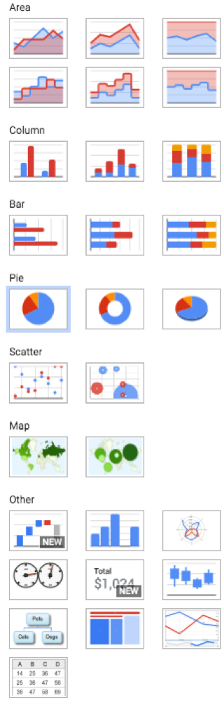
Google Sheets charts are simpler, with less granular control over elements in the chart. All of the major chart types are supported, but you can’t customize them to the same extent as in Excel.
Here’s the list of available chart types in Google Sheets:
Pivot Charts
Google Sheets does not have pivot charts like Excel.
You can create charts directly off pivot data, but if you change the pivot table layout you’ll have to update your chart.
Dynamic Charts
In Excel, if you build a chart from data in an Excel Table then it’s dynamic. If you add data to the table then the chart automatically updates to reflect that. You can also create dynamic named ranges using formulas (principally the OFFSET function), however this method is not available either because you can’t use formulas in named ranges in Google Sheets.
To create dynamic charts in Google Sheets, you leave the chart data range reference open by not specifying an end row, e.g. A1:D instead of A1:D75
You’ll notice that Google Sheets then rebases the range reference to the last row of your Sheet (typically row 1000) so you can update that if needed.
Google Sheet Dashboards
If you decide to build dashboards in Google Sheets, then there are two helpful features.
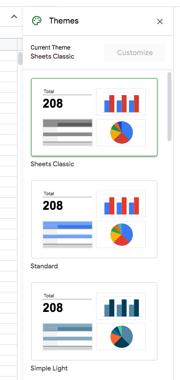
You can add Themes to your Sheet to control the colors of all the charts and pivot tables with a single click. Themes are found under the Format > Theme menu option.
You can choose from a predefined set of templates, or craft your own:
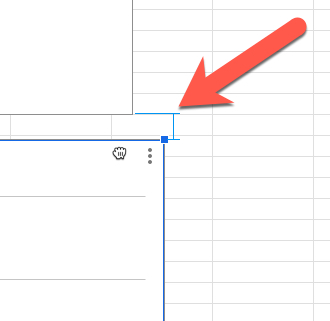
Another useful feature is the alignment feature, that helps you size and line up your charts to match. This is automatically applied, you don’t need to change any settings. You’d be surprised as to how much difference this makes to make your dashboards look professional.
The alignment is shown by a red line:
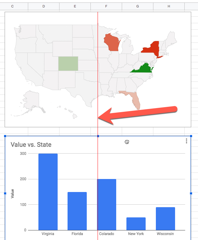
And the sizing feature is shown by blue lines:
My other tip for you is to hide the gridlines (uncheck the option here: View > Gridlines).
Data Studio Dashboards
Google Data Studio is a relatively new tool from Google for building interactive dashboards and beautiful reports.
It’s Google’s answer to Microsoft’s PowerBI tool.
It’s unique selling point is that it’s very easy to use and it’s quick to build professional-looking reports. It works equally well with tiny datasets in Google Sheets or gigantic datasets in BigQuery, as well as a whole host of data from web services (through community connectors).
It’s a fantastic tool.
For many scenarios, it’s a superior tool for building dashboards than just using Google Sheets (which although more flexible is also more finicky).
OTHER DIFFERENCES
Other Differences
Conditional Formatting
In Google Sheets, you cannot:
- Use Databars and Icon sets in conditional formatting
3-D Ranges
Excel has 3-D Ranges, where you apply a formula to the same cell or range across multiple tabs with condensed syntax:
=SUM( A:D!C4 )
is not possible in Google Sheets.
To achieve the same result in Google Sheets, you have to explicitly include the reference for each tab:
=SUM(A!C4, B!C4, C!C4, D!C4)
User Interface Elements
Google Sheets has checkboxes but it does not have spin buttons, scrollbars, option buttons, combo boxes and group list boxes.
For more information on checkboxes in Google Sheets, see:
Miscellaneous Missing Features
- You can’t cut and insert+paste a row or column in Google Sheets
- The new Geography and Stock data types in Excel do not have direct equivalents in Google Sheets
Add-Ins / Add-Ons
Google Sheets calls third-party extensions Add-Ons instead of Add-Ins.
I’ve mentioned a couple of useful Add-Ons for working with data tables in the Working With Data section above.
MACROS, VBA & APPS SCRIPT
Macros, VBA And Apps Script
Macros
Excel and Google Sheets both have the ability to record actions as a macro.
Macros are small programs you create in Excel and Google Sheets, without needing to write any code. They allow you to automate repetitive tasks. They work by recording your actions as you do something and saving these actions as a “recipe” that you can re-use again with a single click.
For example, you can automate formatting tables, creating charts, or doing specific calculations.
For more information about Macros, see:
- The Complete Guide to Simple Automation using Google Sheets Macros, which is chock full of useful macro examples you can copy
- Lesson 2 of the free, introductory Apps Script Blastoff course
VBA And Apps Script
Apps Script is to Google Sheets what VBA is to Excel. Namely a scripting language that lets you extend the functionality of your spreadsheets way beyond what they do natively.
Excel uses the VBA — Visual Basic for Applications — scripting language to record macros and create customized functionality.
Google Sheets, and G Suite, uses Apps Script, a derivative of the JavaScript language, to record macros and automations. Again, you can use it to create custom solutions around Google Sheets.
Since Apps Script is based on JavaScript, you’ll need to learn a new language if you’re coming from an Excel VBA world.
It is very different and will feel strange at first.
There is not a one-to-one relationship between operations and the way each functions.
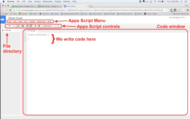
? Starting Apps Script
From inside your Google Sheet, click the menu Tools > Script editor… to open a new tab, which is the Google Apps Script editor window:
You might write a very basic first script like this:
function logTimeRightNow() {
  var timestamp = new Date();
  Logger.log(timestamp);
}
When you run this script in the editor window for the first time, you’re prompted to authorize the script and its scopes (what it’s allowed to access).
Once the script is authorized, it’ll run. When you view the logs, View > Show Logs, you’ll see the current time.
Things To Know About Apps Script
- It runs on Google Servers, so it’s not available offline. It also means that Apps Script does not have access to client-specific objects like the DOM (Document Object Model). It has limited built-in user interaction capabilities.
- Scripts attached to a Google Sheet (or Doc, Slide, etc.) are called Container Bound scripts. A solitary script file is called a Standalone script.
- You can have multiple .gs files in an Apps Script project and they are compiled into a single file at run time.
- There are quotas with Apps Script to control how much processing you can do.
- You can set triggers to run your Apps Script functions automatically, with time-driven or event-driven triggers.
- You can publish your Apps Script files to the web as web apps.
- Apps Script has seamless integration with other G Suite and Google Cloud products through built-in services.
- Integration with other Web Services is entirely possible through APIs. Google have published an OAuth library for authenticated connections.
For more information about Apps Script, see:
- My free, introductory Apps Script Blastoff course
- Google Apps Script: A Beginner’s Guide
- Going GAS — From VBA to Google Apps Script book by expert Bruce McPherson
- Google Apps Script Homepage and documentation from Google
SUMMARY
Summary
This guide covers the major differences between Google Sheets and Excel.
By now you have seen:
- Key differences between Excel and Google Sheets
- Major new functions in Google Sheets, including: QUERY, ArrayFormula, IMPORTRANGE, Language functions, IMPORTHTML, REGEX functions
- Advanced Pivot Table features including Grouping, Calculated Fields, Filtering, Slicers
- Options for working with Excel files
- Charts and Dashboards in Google Sheets
- Dashboards with Google Data Studio
- Macros, custom functions and Apps Script
Next Steps
- Keep learning and stay positive 🙂
- Bookmark this guide for easy reference.
- Sign up for my weekly Google Sheets tips newsletter (your Monday morning espresso in Google Sheets form).
- Take a look at my workshop packages or online courses.
- Get in touch to see how we might work together as you transition from Excel to Google Sheets.
One suggestion on the GAS vs VBA section is to mention that a limitation of GAS (as a server sided script) is that it cannot mimic keystrokes, mouse cursor movements, or use sendkeys. This is a major reason why my organization still relies on Excel macros. In some cases, we have to use “screen scraping” macros to collect data, but in other cases we need to perform repetitive tasks in legacy green-screen applications using sendkeys.
Thanks, Chris! This is a great point.
One of my favorite features of Google Sheets over Excel is that I can literally delete unused rows and columns so I don’t have to worry about defining the last row/column of data in the magical/invisible way you have to in Excel. I can’t tell you how many times I’ve tried to paste a short (maybe 10-20) column of values from Excel into email by copying the column, only to spend a lot of time waiting for my email which is trying to absorb thousands of blank lines at the bottom and then having to ctl-z it and try again with a more mouse-annoying controlled copy. I never have that problem in Google, because it’s now an automatic part of my routine to delete all unused rows and columns and I even have a little script to do that for me, if I remember to use it. This problem alone is near the top of my “why I hate Excel” list.
Yes! It’s a good habit to remove the unused rows/columns to speed up the Sheet too. Hadn’t thought of this additional benefit! Thanks for sharing.
The Functions query and filter alone makes Googlesheets very powerful and versatile compared to Excel. Query brings database-style search to your sheets. But the current limit of 5 million cells is restrictive for large data set analysis, how I hope they increase it to some 20 million at least.
Yes, those two functions are amazing!
And yes, more cells would be helpful. I think it’s something the Google Sheets team are working on.
Very useful summary.
For those who use math formulas, I haven’t found a way to insert math formulas in Google Sheets, similar to what I can do in Excel with Insert Equation. Is there a way to do this?
Hi Larry,
You can use an add-on called Equatio to add math formulas: https://www.texthelp.com/en-us/products/equatio/
Hope this helps!
Ben